![]()
You can run this notebook in a live session or view it on Github.
Using the simplest possible power parameterisation
Create a random trajectory
[1]:
import numpy as np
import pandas as pd
[2]:
np.random.seed(12345)
[3]:
N_points = 100

trajectory = pd.DataFrame(dict(
    u_ship_og=12 + 0.1 * np.random.normal(size=(N_points, )),
    v_ship_og=3 + 0.1 * np.random.normal(size=(N_points, )),
    u_current=2.0 * np.random.normal(size=(N_points, )),
    v_current=2.0 * np.random.normal(size=(N_points, )),
))
[4]:
display(trajectory)
| u_ship_og | v_ship_og | u_current | v_current | |
|---|---|---|---|---|
| 0 | 11.979529 | 2.843434 | 2.254962 | 3.494467 |
| 1 | 12.047894 | 2.943746 | -1.136727 | -2.820492 |
| 2 | 11.948056 | 2.996734 | 0.618724 | -0.756483 |
| 3 | 11.944427 | 2.907099 | -1.154771 | -0.691641 |
| 4 | 12.196578 | 2.951743 | -2.337268 | 0.760125 |
| ... | ... | ... | ... | ... |
| 95 | 12.079525 | 3.091098 | -0.451048 | 0.262203 |
| 96 | 12.011811 | 2.897910 | 2.699452 | -1.395228 |
| 97 | 11.925147 | 2.858658 | 2.700599 | 2.671299 |
| 98 | 12.058497 | 3.129661 | -0.773307 | -0.302078 |
| 99 | 12.015268 | 3.025228 | 1.731979 | 0.885876 |
100 rows × 4 columns
Estimate power needed to maintain speed over ground
[5]:
from rasmus_fuel.simplest import power_maintain_sog, power_to_fuel_burning_rate
[6]:
coefficient = 1.0
[7]:
trajectory["power"] = power_maintain_sog(**trajectory, coeff=coefficient)
[8]:
trajectory["fuel_rate"] = power_to_fuel_burning_rate(trajectory["power"])
[9]:
display(trajectory)
| u_ship_og | v_ship_og | u_current | v_current | power | fuel_rate | |
|---|---|---|---|---|---|---|
| 0 | 11.979529 | 2.843434 | 2.254962 | 3.494467 | 1117.364353 | 0.000053 |
| 1 | 12.047894 | 2.943746 | -1.136727 | -2.820492 | 2529.913503 | 0.000120 |
| 2 | 11.948056 | 2.996734 | 0.618724 | -0.756483 | 1749.777352 | 0.000083 |
| 3 | 11.944427 | 2.907099 | -1.154771 | -0.691641 | 2267.591153 | 0.000108 |
| 4 | 12.196578 | 2.951743 | -2.337268 | 0.760125 | 2700.526265 | 0.000129 |
| ... | ... | ... | ... | ... | ... | ... |
| 95 | 12.079525 | 3.091098 | -0.451048 | 0.262203 | 2056.733168 | 0.000098 |
| 96 | 12.011811 | 2.897910 | 2.699452 | -1.395228 | 1274.605855 | 0.000061 |
| 97 | 11.925147 | 2.858658 | 2.700599 | 2.671299 | 1019.888809 | 0.000049 |
| 98 | 12.058497 | 3.129661 | -0.773307 | -0.302078 | 2197.932609 | 0.000105 |
| 99 | 12.015268 | 3.025228 | 1.731979 | 0.885876 | 1365.750152 | 0.000065 |
100 rows × 6 columns
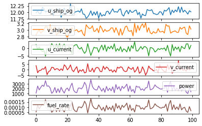
[10]:
trajectory.plot(subplots=True);